1.
Objective
The objective
of this work is developing a generic simulated annealing (SA) algorithm to
solve the traveling salesman problem (TSP), which is find the shortest route
through N given cities such that every city is visited exactly once.
2.
Concepts and Programming
Simulated
annealing algorithm, first described by
Scott Kirkpatric [2], has its name and inspiration come
from annealing in metallurgy, a technique involving heating and slowly
cooling of a material to increase physical strength and/or reduce defects. When
the temperature is hot, the atoms of the material piece gain high
energy and wander randomly. The slow cooling gives them more chances of finding
configurations with lower internal energy than the initial one [3]. In term of
an optimization algorithm, each step of the SA algorithm replaces the current
solution by a random "neighbor" solution, chosen with a probability
that depends both on the difference between the corresponding function values
(energy) and also on a global parameter T (called
the temperature). The temperature is gradually decreased during the
process. At the beginning, T is large, the "upnhill" moves
(go to higher energy states) are more likely accepted than when T is go to zero
at the end of the process. This allows the SA algorithm move out of the local
minimum at the early states.
Table 1: Pseudo
code of SA algorithm [2]
s ← s0; // Initial state, energy.
e ← E(s)
sbest ← s; // "best"
solution
ebest ← e
k ← 0
while k < kmax and e > emax
// Trail move to ‘ neighbor’
snew ← neighbor(s)
enew ← E(snew)
// Accept uphill move if ‘feel lucky’
if
P(e, enew, temp(k/kmax)) > random() then
s ← snew;
e ← enew; end // Tracking the best-ever
if enew < ebest then
sbest ← snew;
ebest ← enew end
k ← k + 1
return sbest
|
There are different schemes to accept the “uphill”
move as well as to reduce the temperature, such as Fast Cauchy, Geometric, or
Boltzmann’s methods as given in [1]- lecture 3, page 5.
Actually, the "pure" SA algorithm as
described in [1] does not keep track of the best solution found so far: it does
not use the variables sbest and ebest, it lacks the
second if inside the loop, and, at the end, it returns the current
state s instead of sbest. While remembering the best state is a
standard technique in optimization that can be used in any meta-heuristic, it
does not have an analogy with physical annealing — since a physical system can
"store" a single state only.
In TSP problem:
- Each state “s” is represented by a combinatory of N
cities’ indexes.
- The energy E(s) is a function to compute the total
travel distance of visiting N cities following the route or the state s.
- The initial sate or route s is selected randomly.
- The “neighbor” of s is implemented by swapping 2
random cities of the route s. There are 2 ways to swap: swap the two vertices
or swap the two edges as described in [1]-lecture 3, page 17, and are both
implemented in my code (See Code listing section)
- The probability to accept a move is P = exp(- DE/kT) = exp(-(enew-e)/kT)
- Update temperature T = αT, where 0<α<1
3. Some Results
 |
| SA process |
 |
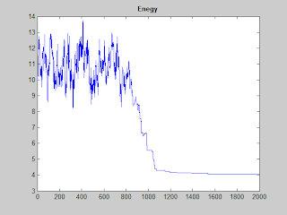
| The convergence of SA |
 |
| GUI (Graphic User Interface) written in Matlab |
http://www.mathworks.com/matlabcentral/fileexchange/9612-traveling-salesman-problem-tsp-using-simulated-annealing . So what the difference?
Main thing is the speed. I am inspired by his work, but after downloaded, I found that his program could take "forever" for 101 cities. Could not sit and wait, (not a patient person) so I wrote this program. Most of the time, it just needs less than 10 seconds for 101 cities (including time for plot). For 500 cities, it may take 1 minutes.
Next time, I will upload the code and talk about using SA for solving N-Queens problem.
References
1.
Gary Yen. ECEN
5773 Intelligent Systems- Fall 2011 lecture notes. Oklahoma State University,
2011
2. Kirkpatrick, S., C. D.
Gelatt Jr., M. P. Vecchi, "Optimization by Simulated Annealing",Science, 220, 4598, 671-680, 1983.